Demo SensorAffinity.

Examples

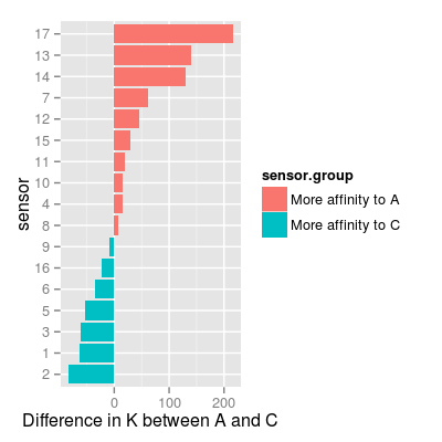
# define a representative set of gases A, C and AC 
# - appropriate to test sensor affinities across two species A and C
set <- c("A 0.01", "A 0.05", "C 0.1", "C 1", "A 0.01, C 0.1", "A 0.05, C 1")

# 0) check UNIMAN sensors and their sorption affinities
data(UNIMANsorption)

df <- as.data.frame(UNIMANsorption$qkc[, , "K"])
head(df)

         A        B         C
1 53.64473 46.02505 117.11543
2 62.88488 46.75066 146.01511
3 50.67575 44.31645 111.97059
4 80.66829 33.66036  65.54146
5 50.28884 42.04818 104.33481
6 90.60876 39.36334 126.07980


df <- mutate(df,
  sensor = 1:nrow(df),
  sensor.group = ifelse(A > C, "More affinity to A", "More affinity to C"))

p <- ggplot(df, aes(reorder(x = factor(sensor), A - C), y = A - C, fill = sensor.group)) + 
  geom_bar(position = "identity") + coord_flip() +
  xlab("sensor") + ylab("Difference in K between A and C")
p

Mapping a variable to y and also using stat="bin".
  With stat="bin", it will attempt to set the y value to the count of cases in each group.
  This can result in unexpected behavior and will not be allowed in a future version of ggplot2.
  If you want y to represent counts of cases, use stat="bin" and don't map a variable to y.
  If you want y to represent values in the data, use stat="identity".
  See ?geom_bar for examples. (Deprecated; last used in version 0.9.2)

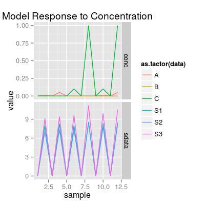
# in result:
# - sensors with affinities A > C: 17, 13, 14, ...
# - sensors with affinities C > A: 2, 1, 3, ...

# 1) sensors with affinities A > C
# - set drift noise level 'dsd' to zero, 
#   in order to see more a class-relevant information, than drift
sa1 <- SensorArray(num = c(13, 14, 17), dsd = 0)

# look at the level of signal in reponse to pure analytes and to a mixture
# - it is important, as 
#  1) PCA mostly captures a variation in the absolute level of signals
#  2) accroding to the models for data geenration, mixture response is 
#     a sum of responses to pure analytes (mixture is composed of),
#     thus, absolute values of signals matter.
p0 <- plotSignal(sa1, set = set)
p0



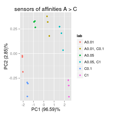
p1 <- plotPCA(sa1, set = rep(set, 3), air = FALSE, main = "sensors of affinities A > C")
p1



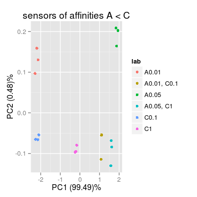
# 2) sensors with affinities A < C
sa2 <- SensorArray(num = 1:3, dsd = 0) 

p2 <- plotPCA(sa2, set = rep(set, 3), air = FALSE, main = "sensors of affinities A < C")
p2



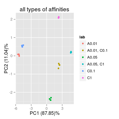
# 3) all available 17 types of sensors
sa3 <- SensorArray(num = 1:17, dsd = 0)

p3 <- plotPCA(sa3, set = rep(set, 3), air = FALSE, main = "all types of affinities") 
p3