DriftNoiseModel-class. chemosensors 0.7.7

Usage

DriftModelNames()

defaultParDriftNoiseModel()

DriftNoiseModel(...)

Arguments

...: parameters of constructor.

Value

Character vector of model names.

List of the default parameters.

Description

Method ndcomp.

Method ndvar.

Method dspace.

Class DriftNoiseModel generates the drift noise in a multi-variate manner in several steps.

Function to get model names of class DriftNoiseModel.

Function to get default constructor parameters of class DriftNoiseModel.

Constructor method of DriftNoiseModel Class.

Wrapper function DriftNoiseModel.

Details

The primary question arising in drift modeling is related to the way of one defines the drift phenomena for gas sensor arrays. We propose to evaluate a drift subspace via common principal component analysis. The hypothesis of common principal component analysis states that exists an orthogonal matrix V such that the covariance matrices of K groups have the diagonal form simultaneously. The resulted eigenvectors (columns of the matrix V) define the subspace common for the groups and orthogonal across the components.

A preliminary step involves quantification of drift-related data presented in the long-term UNIMAN dataset. These results are stored in UNIMANdnoise dataset.

On the next step the drift is injected in the sensor array data by generating the noise by multi-dimensional random walk based on the multivariate normal distribution with zero-mean and diagonal covariance matrix - in the sub-space defined by the matrix V. The relative proportion along the diagonal elements in the covariance matrix is specified by the importance of drift components in terms of of projected variance.

On the final step the component correction operation is recalled to induce the generated noise from the random walk back into the complete multivariate space of the sensor array data.

Slots of the class:

`num`	Sensor number (`1:17`), which drift profile is used. The default value is `c(1, 2)`.
`dsd`	Parameter of standard deviation used to generate the drift noise. The deault value is 0.1.
`ndcomp`	The number of components spanning the drift sub-space. The default number is 2.
`ndvar`	The importance values of drift components. The default values are `UNIMANdnoise` dataset.
`driftModel`	Drift model of class `DriftCommonModel`.

Methods of the class:

`predict`	Generates multi-variate noise injeted to an input sensor array data.
`dsd`	Gets the noise level.
`dsd<-`	Sets the noise level.

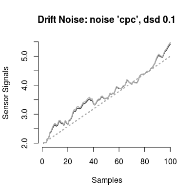
The plot method has three types (parameter y):

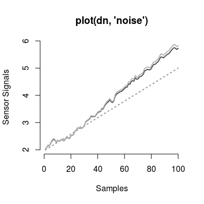
`noise`	(default) Depicts the drift noise generated by the model with a linechart.
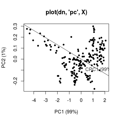
`pc`	Shows the drift components in a PCA scoreplot of an input sensor array data (parameter `X`.

Note

In the case num is different from value c(1:17), the number of components is not the same as in V matrix. First, the colums in V matrix are selected according to numbers pointed in num. Second, QR-decomposition of the resulted matrix is performed to orthogonolize the component vectors.

Examples

# model: default initialization
dn <- DriftNoiseModel()

# get information about the model
show(dn)

 Drift Noise Model (dsd 0.1), common model 'cpc'

print(dn)

 Drift Noise Model
 - num 1, 2 
 drift common model
 - method: cpc 
 - ndcomp: 1 


plot(dn)  



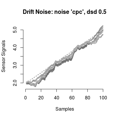
# model: custom parameters
# - many sensors
dn <- DriftNoiseModel(dsd=0.5, ndcomp=3, num=1:17)

print(dn)

 Drift Noise Model
 - num 1, 2, 3 ... 17 
 drift common model
 - method: cpc 
 - ndcomp: 3 


plot(dn)



# method plot
#  - plot types 'y': barplot, noise, walk
dn <- DriftNoiseModel() # default model

plot(dn, "noise", main="plot(dn, 'noise')") 


# default plot type, i.e. 'plot(dn)' does the same plotting

data(UNIMANshort)
X <- UNIMANshort$dat[, num(dn)]
plot(dn, "pc", X, main="plot(dn, 'pc', X)")



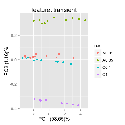
### example with a SensorArray
set.seed(1)
sa <- SensorArray(num = 1:5)

set <- c("A 0.01", "A 0.05", "C 0.1", "C 1")
sc <- Scenario(rep(set, 10))
conc <- getConc(sc)

sdata <- predict(sa, conc)

p1 <- plotPCA(sa, conc = conc, sdata = sdata, air = FALSE, 
  main = "feature: transient")
p1



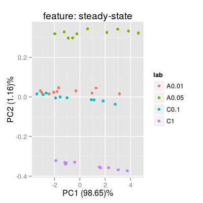
p2 <- plotPCA(sa, conc = conc, sdata = sdata, feature = "ss", 
  main = "feature: steady-state")
p2



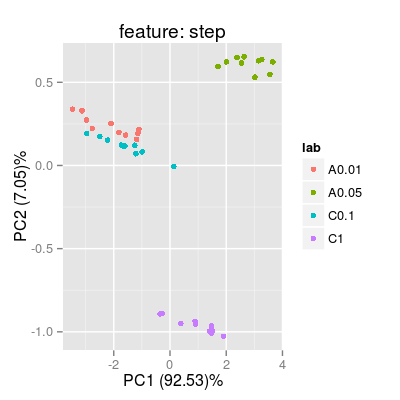
p3 <- plotPCA(sa, conc = conc, sdata = sdata, feature = "step", 
  main = "feature: step")
p3