Demo NeuromorphicSim.

Examples

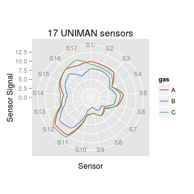
# Many lines of code are commented to respect the CRAN policy on CPU time per Rd file.

# options(cores = 2) 
# use this option to confiure the parallel computation 
# (in this case 2 CPU cores are specified)

### step 1/7: take a look at the reference array of 17 UNIMAN sensors
sa.uniman <- SensorArray(nsensors = 17) 

# polar plot 
plot(sa.uniman, 'polar', main = "17 UNIMAN sensors")



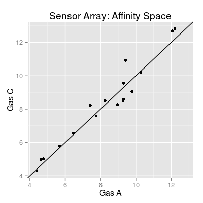
# affinity space for gases 1 and 3
plot(sa.uniman, 'affinitySpace', gases = c(1, 3))



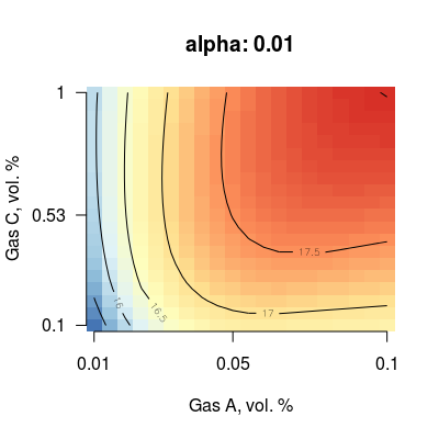
### step 2/7: select sensor non-linearity (parameter alpha) for a sensor
# - (here) sensor `num` is 3, tesed values of `alpha` are 0.01, 1 and 2.25
# - (note) in the current implementation, parameter `alpha` is the same 
#    for all sensors in a array
s <- Sensor(num = 3, alpha = 0.01)
plotMixture(s, gases = c(1, 3), main = paste("alpha:", alpha(s)))



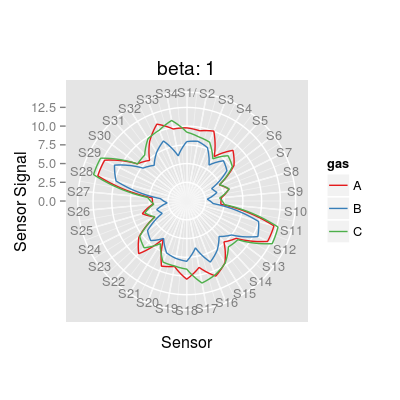
#s <- Sensor(num = 3, alpha = 1)
#plotMixture(s, gases = c(1, 3), main = paste("alpha:", alpha(s)))

#s <- Sensor(num = 3, alpha = 2.25)
#plotMixture(s, gases = c(1, 3), main = paste("alpha:", alpha(s)))

### step 3/7: select sensor diversity (parameter beta) for a sensor array
# - (here) the number of sensors `nsensors` is 34 (two times more than 17 UNIMAN sensors)
#    tesed values of `beta` are 1, 2, 5 and 10
sa <- SensorArray(nsensors = 34, beta = 1)
plot(sa, 'polar', main = paste("beta:", beta(sa)))



#sa <- SensorArray(nsensors = 34, beta = 2)
#plot(sa, 'polar', main = paste("beta:", beta(sa)))

#sa <- SensorArray(nsensors = 34, beta = 5)
#plot(sa, 'polar', main = paste("beta:", beta(sa)))

#sa <- SensorArray(nsensors = 34, beta = 10)
#plot(sa, 'polar', main = paste("beta:", beta(sa)))

### step 4/7: define the parameters of the array
# - (here we use the default parameters) 
#   `alpha` is 2.25 (default), `beta` is 2,
#   noise parameters `csd`, `ssd` and `dsd` are all 0.1,
sa <- SensorArray(nsensors = 34)

# polar plot
#plot(sa, 'polar', main = "Virtual sensors")

# affinity space for gases 1 and 3
#plot(sa, 'affinitySpace', gases = c(1, 3))

### step 5: define a concentration matrix (via class Scenario)
# - (here) let's assume a scenario of mixture quantification for gases 1 and 3 
#   `tunit` is set to 60 (recommended value)
training.set <- c("A 0.01", "A 0.05", "C 0.1", "C 1")
validation.set <- c("A 0.01, C 0.1", "A 0.0025, C 0.5", "A 0.05, C 1")

sc <- Scenario(tunit = 60, T = training.set, nT = 2, V = validation.set, nV = 2)

#plot(sc)
#plot(sc, facet = FALSE, concUnits = 'norm')

# extract conc. matrix
conc <- getConc(sc)

print(head(conc))

  A B C
1 0 0 0
2 0 0 0
3 0 0 0
4 0 0 0
5 0 0 0
6 0 0 0


### step 6/7: generate sensor data in reaction to `conc`
conc0 <- conc[1:240, ] 
# to save CPU time of demonstration, 
# we use just two cycles of 2x60 time length each
# 1 cycle = gas exposure phase and cleaning phase

#sdata <- predict(sa, conc0, nclusters = 2)

#p1 <- qplot(X1, value, data = melt(sdata), geom = "line") + facet_wrap(~ X2) + 
#  xlab("Time, a.u.") + ylab("Sensor Signal, a.u.")

### step 7/7: some additional plots for testing

# plot just few sensors
#p2 <- qplot(X1, value, data = melt(sdata[, 1:2]), geom = "line") + facet_wrap(~ X2) + 
#  labs(x = "Time, a.u.", y = "Sensor Signal, a.u.", title = "First two sensors")

# re-generate sensor data as noise-free
sa0 <- sa
csd(sa0) <- 0
ssd(sa0) <- 0
dsd(sa0) <- 0
sa0

 Sensor Array of 34 sensors, 3 gases A, B, C
 - enableSorption TRUE, enableDyn FALSE
 - Sensor Model (num 1, 2, 3 ... 17), beta 2, data model 'ispline'
 - Sorption Model (knum 1, 2, 3 ... 17), alpha 2.25
 - Concentration Noise Model (csd 0), noise type 'logconc'
 - Sensor Noise Model (ssd 0), noise type 'randomWalk'
 - Drift Noise Model (dsd 0), common model 'cpc'


#sdata0 <- predict(sa0, conc0, nclusters = 2) 

#p3 <- qplot(X1, value, data = melt(sdata0), geom = "line") + facet_wrap(~ X2) + 
#  labs(x = "Time, a.u.", y = "Sensor Signal, a.u.", title = "Noise-free array")